Brief of Data-Structure & Algorithm (DSA) coding interview questions

Some concepts, topics, and examples for Leetcode coding interview

2026 · coding interview · dsa

Practice platforms

More of my implementations can be found here: Github: quanhn232/LeetCode

DSA coding interview template

REPHRASE the question: in your own words -> make sure you understand the question correctly
CONSTRAINTS: clarify input and output (size, type) and any ambiguity
Walkthrough 1 - 2 EXAMPLES (this helps with brainstorm ideas / intuition)
INTUITION (thinking time is here, note down your thoughts): observations -> what DSA to use, main logics, time / space analysis
CODE
TEST: be active in testing, don’t wait for interviewer to ask you to

https://www.youtube.com/watch?v=dRmdp1q2DXM

Prefix sum

Practice problems

238. Product of Array Except Self
303. Range Sum Query - Immutable
304. Range Sum Query 2D - Immutable
325. Maximum Size Subarray Sum Equals k (with Hashmap)
523. Continuous Subarray Sum (with Hashmap)
525. Contiguous Array (with Hashmap)
548. Split Array with Equal Sum
724. Find Pivot Index
930. Binary Subarrays With Sum
974. Subarray Sums Divisible by K
1248. Count Number of Nice Subarrays (with Hashmap)
1413. Minimum Value to Get Positive Step by Step Sum
1590. Make Sum Divisible by P
1658. Minimum Operations to Reduce X to Zero (with Hashmap)
1983. Widest Pair of Indices With Equal Range Sum

Map/Set

Practice problems

Big num

Practice problems

2D array

Practice problems

Sliding window

Patterns

Template:


1
2
3
4
5
6
 def sliding_window(nums):
    1. Iterate over elements in our input == Expand the window (left, right)
    2. Meet the condition to stop expansion - the most difficult part
        2.1. Remove nums[left] from window
        2.2. Contract the window
    3. Process the current valid  window

Notes:

Sliding windows with 2 pointers works when the problem has monotonic properties - meaning that expanding the window consistently moves us in one direction regarding our constraint, and shrinking consistently moves us in the opposite direction.
Key Criteria for Two Pointers/Sliding Window (Both should be True) (sliding window vs DP):
1. Rule 1 (Validity of Wider Scope): If a larger window (wider scope) is valid, all smaller sub-windows within it must also be valid.
2. Rule 2 (Invalidity of Narrower Scope): If a smaller window (narrower scope) is invalid, all larger windows containing it must also be invalid.

Sources:

https://leetcode.com/discuss/post/6900561/ultimate-sliding-window-guide-patterns-a-28e9/
https://adamowada.github.io/leetcode-study/sliding-window/study-guide.html
https://github.com/0xjaydeep/leetcode-patterns/blob/main/patterns/sliding_window/README.md

Practice problems

Greedy

Reference:

https://medium.com/algorithms-and-leetcode/greedy-algorithm-explained-using-leetcode-problems-80d6fee071c4

Practice problems

Activity-Selection

given a set of activities with start and end time (s, e), our task is to schedule maximum non-overlapping activities or remove minimum number of intervals to get maximum non-overlapping intervals. In cases that each interval or activity has a cost, we might need to retreat to dynamic programming to solve it.

Practice problems

Frog Jumping

Practice problems

Data Compression

Practice problems

File Merging

Practice problems

Graph Algorithms

Minimum Spanning Tree (Kruskal’s or Prim’s)
Dijkstra
Bellman-Ford

Binary search

Instruction

Reference:

https://medium.com/swlh/binary-search-find-upper-and-lower-bound-3f07867d81fb
https://leetcode.com/explore/learn/card/binary-search/136/template-analysis/935/

Templates

Usually I prefer following template #2

Template #1 (left <= right):
- Most basic and elementary form of Binary Search
- Search Condition can be determined without comparing to the element’s neighbors (or use specific elements around it)
- No post-processing required because at each step, you are checking to see if the element has been found. If you reach the end, then you know the element is not found
Template #2 (left < right):
- An advanced way to implement Binary Search.
- Search Condition needs to access the element’s immediate right neighbor
- Use the element’s right neighbor to determine if the condition is met and decide whether to go left or right
- Guarantees Search Space is at least 2 in size at each step
- Post-processing required. Loop/Recursion ends when you have 1 element left. Need to assess if the remaining element meets the condition.

Choosing Mid, Left, Right

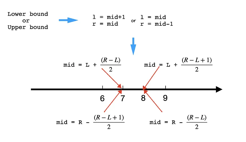
Pick the mid: Pick the former one or the latter one out of an even number of items. Both of them works, but it should align with how we deal with l and r. When we select the former one using l+(r-l)/2, we want to make sure to avoid l = mid because that might lead to infinite loop. For example when there are two elements [0,1] and mid = 0, then l becomes mid and the iteration goes again and again. Similarly, when we select the latter one using r-(r-l)/2, we want to avoid r = mid.

Assign values to L and R:

For example, when the question asks for the lower bound:

if mid works, then r should be mid not mid-1 because mid might be the answer!
And when mid does not work, l should be mid+1 because we are sure the mid is not the answer and everything falls one mid’s left won’t work either.

Assign L and R when asked for the lower bound.


1
2
3
4
5
6
7
8
 def binary_search_lower(nums, target, expect):
    while left < right:
      mid = left + (right - left) // 2 # lower bound, since mid=l+(r-l)/2, we must avoid l = mid (infinite loop, e.g. arr=[0,1] with target=0)
      if condition(mid): # if mid works
          right = mid
      else:
          left = mid + 1 # otherwise causes infinite loop
    return left # find left most index (left == right)

For example, when the question asks for the upper bound:

if mid does not work, r should be mid-1 because we are sure the mid is not the answer and everything falls one mid’s right won’t work either.
And when mid works, then l should be mid not mid-1 because mid might be the answer!

Assign L and R when asked for the upper bound.


1
2
3
4
5
6
7
8
 def binary_search_upper(nums, target, expect):
    while left < right:
        mid = right - (right - left) // 2
        if condition(mid): # if mid works
            right = mid - 1
        else:
            left = mid
    return left

Basic

Practice problems

Modified

Practice problems

Adhoc binary search

Practice problems

Matrix

Practice problems

Hard

Practice problems

4. Median of Two Sorted Arrays

Tree

Reference:

https://leetcode.com/discuss/post/3743769/crack-easily-any-interview-tree-data-str-nxr9/
https://www.geeksforgeeks.org/dsa/preorder-vs-inorder-vs-postorder/
https://cp-algorithms.com/

Basic

Traversal

Suppose this definition for a binary tree node:

 class TreeNode:
    def __init__(self, val: int=0, left: TreeNode=None, right: TreeNode=None):
        self.val = val
        self.left = left
        self.right = right
 

Morris Traversal Template & Explanation (inorder example)

Step 1: Initialize current as root

Step 2: While current is not NULL,

  If current does not have left child
     a. Add current’s value
     b. Go to the right, i.e., current = current.right
 Else
     a. In current's left subtree, make current the right child of the rightmost node
     b. Go to this left child, i.e., current = current.left
 

Example:

First, 1 is the root, so initialize 1 as current, 1 has left child which is 2, the current’s left subtree is

So in this subtree, the rightmost node is 5, then make the current(1) as the right child of 5. Set current = current.left (current = 2). The tree now looks like:

For current 2, which has left child 4, we can continue with the same process as we did above

then add 4 because it has no left child, then add 2, 5, 1, 3 one by one, for node 3 which has left child 6, do the same as above. Finally, the inorder traversal is [4,2,5,1,6,3].

Inorder Traversal


1
2
3
4
5
6
7
8
 def inorderTraversal(root: TreeNode, res: List[TreeNode]) -> List[int]:
    """Time: O(n); Space: O(n)
    """
    if root is None: return

    inorderTraversal(root.left, res)
    res.append(root.val)
    inorderTraversal(root.right, res)


1
2
3
4
5
6
7
8
9
10
11
12
13
14
15
16
 def inorderTraversal(root: TreeNode) -> List[int]:
    """Time: O(n); Space: O(n)
    """
    res, stack = [], []
    curr = root

    while curr or stack:
        while curr:
            stack.append(curr)
            curr = curr.left

        curr = stack.pop()
        res.append(curr.val)
        curr = curr.right

    return res


1
2
3
4
5
6
7
8
9
10
11
12
13
14
15
16
17
18
19
20
21
22
23
24
 def inorderTraversal(root: TreeNode) -> List[int]:
    """Time: O(n); Space: O(1)
    """
    res = []
    curr = root

    while curr is not None:
        if curr.left is None:
            res.append(curr.val)
            curr = curr.right
        else:
            pred = curr.left
            while pred.right is not None and pred.right is not curr:
                pred = pred.right

            if pred.right is None:
                pred.right = curr
                curr = curr.left
            else:
                pred.right = None
                res.append(curr.val)
                curr = curr.right

    return res

Practice problems

94. Binary Tree Inorder Traversal

Preorder Traversal


1
2
3
4
5
6
7
8
 def preorderTraversal(root: TreeNode, res: List[TreeNode]) -> List[int]:
    """Time: O(n); Space: O(n)
    """
    if root is None: return
    
    res.append(root.val)
    preorderTraversal(root.left, res)
    preorderTraversal(root.right, res)


1
2
3
4
5
6
7
8
9
10
11
12
13
14
15
16
 def preorderTraversal(root: TreeNode) -> List[int]:
    """Time: O(n); Space: O(n)
    """
    res, stack = [], []
    curr = root

    while curr or stack:
        while curr:
            res.append(curr.val)
            stack.append(curr)
            curr = curr.left

        curr = stack.pop()
        curr = curr.right

    return res


1
2
3
4
5
6
7
8
9
10
11
12
13
14
15
16
17
18
19
20
21
22
23
24
 def preorderTraversal(root: TreeNode) -> List[int]:
    """Time: O(n); Space: O(1)
    """
    res = []
    curr = root

    while curr is not None:
        if curr.left is None:
            res.append(curr.val)
            curr = curr.right
        else:
            pred = curr.left
            while pred.right is not None and pred.right is not curr:
                pred = pred.right

            if pred.right is None:
                res.append(curr.val)
                pred.right = curr
                curr = curr.left
            else:
                pred.right = None
                curr = curr.right

    return res

Practice problems

Postorder Traversal


1
2
3
4
5
6
7
8
 def postorderTraversal(root: TreeNode, res: List[TreeNode]) -> List[int]:
    """Time: O(n); Space: O(n)
    """
    if not root: return
    
    postorderTraversal(root.left, res)
    postorderTraversal(root.right, res)
    res.append(root.val)


1
2
3
4
5
6
7
8
9
10
11
12
13
14
15
16
 def postorderTraversal(root: TreeNode) -> List[int]:
    """Time: O(n); Space: O(n)
    """
    res, stack = [], []
    curr = root

    while curr or stack:
        while curr:
            res.append(curr.val)
            stack.append(curr)
            curr = curr.right

        curr = stack.pop()
        curr = curr.left

    return res[::-1]


1
2
3
4
5
6
7
8
9
10
11
12
13
14
15
16
17
18
19
20
21
22
23
24
25
26
27
28
29
30
31
32
33
34
35
36
37
38
39
40
41
42
43
44
45
46
47
48
 def postorderTraversal(root: TreeNode) -> List[int]:
    """Time: O(n); Space: O(1)
    """
    def reverse_right(start: TreeNode, end: TreeNode) -> None:
        if start is end:
            return

        prev = None
        curr = start
        while curr is not end:
            nxt = curr.right
            curr.right = prev
            prev = curr
            curr = nxt

        curr.right = prev

    res = []
    dummy = TreeNode(0)
    dummy.left = root
    curr = dummy

    while curr is not None:
        if curr.left is None:
            curr = curr.right
        else:
            pred = curr.left
            while pred.right is not None and pred.right is not curr:
                pred = pred.right

            if pred.right is None:
                pred.right = curr
                curr = curr.left
            else:
                reverse_right(curr.left, pred)

                node = pred
                while True:
                    res.append(node.val)
                    if node is curr.left:
                        break
                    node = node.right

                reverse_right(pred, curr.left)
                pred.right = None
                curr = curr.right

    return res

Practice problems

Level-order Traversal


1
2
3
4
5
6
7
8
9
10
11
12
13
14
15
16
17
18
19
20
 def levelorderTraversal(node): # BFS approach
    # 1. initialize queue for current level
    curr_level_queue = [node]
    
    while curr_level_queue:
        # 2. initialize queue for next level
        next_level_queue = []

        # 3. iter thru all nodes in current level
        while curr_level_queue:
            node = curr_level_queue.popleft()
            # do sth with node

            # 4. add node's children into queue for next level
            next_level_queue.append(node.left)
            next_level_queue.append(node.right)

        # 5. set curr_level_queue = next level to be considered
        curr_level_queue = next_level_queue

Practice problems

Ancestor problems

Common ancestor (e.g: Lowest common ancestor)

Practice problems

Root to leaf path problems

Practice problems

Depth problem

Practice problems

Travel child to parent problems (Radial Traversal)


1
2
3
4
5
6
7
8
9
10
11
 """Template
1. Build parent and child relation map
2. Do level order traversal or DFS
"""
parent = {}
def dfs(root, par):
    if not root: return
    
    parent[root] = par
    dfs(root.left, root)
    dfs(root.right, root)

Practice problems

Tree construction

Practice problems

Serialize and Deserialize tree

Practice problems

Distance between two Nodes

Practice problems

Binary Search Tree (BST)

Practice problems

Validate

Practice problems

Disjoint Set Union (DSU)/Union Find

https://cp-algorithms.com/data_structures/disjoint_set_union.html

Fenwick Tree

https://cp-algorithms.com/data_structures/fenwick.html

Segment Tree

https://cp-algorithms.com/data_structures/segment_tree.html

Trie

Reference:

https://leetcode.com/problems/implement-trie-prefix-tree/

Implementation template:


1
2
3
4
5
6
7
8
9
10
11
12
13
14
15
16
17
18
19
20
21
22
23
24
25
26
27
28
29
30
31
32
33
34
35
36
37
38
39
40
41
42
43
44
45
46
47
48
49
50
51
52
53
 class TrieNode:
    def __init__(self):
        self.children = {}
        self.isEndOfWord = False

class Trie:
    def __init__(self):
        self.root = TrieNode()
        self.root.isEndOfWord = False

    def insert(self, word: str) -> None:
        current = self.root
        for c in word:
            if c not in current.children:
                current.children[c] = TrieNode()
            current = current.children[c]
        current.isEndOfWord = True

    def search(self, word: str) -> bool:
        current = self.root
        for c in word:
            nextNode = current.children.get(c, None)
            if not nextNode: return False
            current = nextNode
        return current.isEndOfWord

    def startsWith(self, prefix: str) -> bool:
        current = self.root
        for c in prefix:
            nextNode = current.children.get(c, None)
            if not nextNode: return False
            current = nextNode
        return True

    def lcs(self):
        ans = []
        current = self.root
        while current:
            if len(current.children) > 1 or current.isEndOfWord:
                break
            else:
                key = list(current.children.keys())
                ans.append(key[0])
                current = current.children.get(key[0])
       
        return ''.join(ans)

    def canBeBuiltByOtherWords(self, word):
        current = self.root
        for c in word:
            current = current.children[c]
            if not current.isEndOfWord: return False
        return True

Practice problems

Graph

References:

https://leetcode.com/discuss/post/3900838/mastering-graph-algorithms-a-comprehensi-xyws/
https://blog.algomaster.io/p/master-graph-algorithms-for-coding

Breadth First Search (BFS)

BFS is a fundamental graph traversal algorithm that systematically explores the vertices of a graph level by level.

Starting from a selected node, BFS visits all of its immediate neighbors first before moving on to the neighbors of those neighbors. This ensures that nodes are explored in order of their distance from the starting node. BFS is particularly useful in scenarios such as:

Finding the minimal number of edges between two nodes.
Processing nodes in a hierarchical order, like in tree data structures.
Finding people within a certain degree of connection in a social network.

Complexity (V: no. of vertices; E: no. of edges):

Time: O(V + E): the algorithm visits each vertex and edge once.
Space: O(V): for the queue and visited set used for traversal.


1
2
3
4
5
6
7
8
9
10
11
12
13
14
15
16
17
 from collections import deque

def bfs(graph, start):
    visited = set()
    queue = deque([start])
    visited.add(start)
    while queue:
        vertex = queue.popleft()
        
        if vertex in visited: continue
        visited.add(vertex)
        # so sth

        for neighbor in graph[vertex]:
            if neighbor not in visited:
                visited.add(neighbor)
                queue.append(neighbor)

Practice problems

Depth First Search (DFS)

DFS is a fundamental graph traversal algorithm used to explore nodes and edges of a graph systematically.

It starts at a designated root node and explores as far as possible along each branch before backtracking. DFS is particularly useful in scenarios like:

Find a path between two nodes.
Checking if a graph contains any cycles.
Identifying isolated subgraphs within a larger graph.
Topological Sorting: Scheduling tasks without violating dependencies.

Complexity (V: no. of vertices; E: no. of edges):

Time: O(V + E): the algorithm visits each vertex and edge once.
Space: O(V): due to stack used for recursion (in recursive implementation) or an explicit stack (in iterative implementation).


1
2
3
4
5
6
7
8
 def dfs(graph, node, visited: set):
    visited.add(node)

    # do sth with node
    
    for neighbor in graph[node]:
        if neighbor not in visited:
            dfs(graph, neighbor, visited)


1
2
3
4
5
6
7
8
9
10
11
 def dfs(graph, start):
    visited = set()
    stack = [start]
    while stack:
        node = stack.pop()
        if node not in visited:
            visited.add(node)
            print(f"Visiting {node}")
            # Add neighbors to stack
            stack.extend([neighbor for neighbor in graph[node] if neighbor not in visited])
    return visited

Practice problems

Topological Sort

Topological Sort algorithm is used to order the vertices of a Directed Acyclic Graph (DAG) in a linear sequence, such that for every directed edge u $\rightarrow$ v, vertex u comes before vertex v in the ordering.

Essentially, it arranges the nodes in a sequence where all prerequisites come before the tasks that depend on them.

Topological Sort is particularly useful in scenarios like:

Determining the order of tasks while respecting dependencies (e.g., course prerequisites, build systems).
Figuring out the order to install software packages that depend on each other.
Ordering files or modules so that they can be compiled without errors due to missing dependencies.

Complexity:

Time: O(V + E) since each node and edge is processed exactly once.
Space: O(V) for storing the topological order and auxiliary data structures like the visited set or in-degree array.


1
2
3
4
5
6
7
8
9
10
11
12
13
14
15
 def topological_sort_dfs(graph):
    visited = set()
    stack = []

    def dfs(vertex):
        visited.add(vertex)
        for neighbor in graph.get(vertex, []):
            if neighbor not in visited:
                dfs(neighbor)
        stack.append(vertex)

    for vertex in graph:
        if vertex not in visited:
            dfs(vertex)
    return stack[::-1]  # Reverse the stack to get the correct order

Explanation:

DFS Traversal: Visit each node and recursively explore its neighbors.
Post-Order Insertion: After visiting all descendants of a node, add it to the stack.
Result: Reverse the stack to obtain the topological ordering.


1
2
3
4
5
6
7
8
9
10
11
12
13
14
15
16
17
18
19
20
21
22
23
 from collections import deque

def topological_sort_kahn(graph):
    in_degree = {u: 0 for u in graph}
    for u in graph:
        for v in graph[u]:
            in_degree[v] = in_degree.get(v, 0) + 1

    queue = deque([u for u in in_degree if in_degree[u] == 0])
    topo_order = []

    while queue:
        u = queue.popleft()
        topo_order.append(u)
        for v in graph.get(u, []):
            in_degree[v] -= 1
            if in_degree[v] == 0:
                queue.append(v)

    if len(topo_order) == len(in_degree):
        return topo_order
    else:
        raise Exception("Graph has at least one cycle")

Explanation:

Compute In-Degrees: Calculate the number of incoming edges for each node.
Initialize Queue: Start with nodes that have zero in-degree.
Process Nodes:
1. Dequeue a node, add it to the topological order.
2. Reduce the in-degree of its neighbors.
3. Enqueue neighbors whose in-degree becomes zero.
Cycle Detection: If the topological order doesn’t include all nodes, the graph contains a cycle.

Practice problems

Union Find (a.k.a Disjoint Set Union - DSU)

Union Find is a data structure that keeps track of a set of elements partitioned into disjoint (non-overlapping) subsets.

It supports two primary operations:

Find (Find-Set): Determines which subset a particular element belongs to. This can be used to check if two elements are in the same subset.
Union: Merges two subsets into a single subset, effectively connecting two elements.

Union Find is especially useful in scenarios like:

Quickly checking if adding an edge creates a cycle in a graph.
Building a Minimum Spanning Tree by connecting the smallest edges while avoiding cycles.
Determining if two nodes are in the same connected component.
Grouping similar elements together.

Complexity:

Time (per Operation): Find and Union: Amortized O(α(n)), where α(n) is the inverse Ackermann function, which is nearly constant for all practical purposes.
Space: O(n), where n is the number of elements, for storing the parent and rank arrays.

How Union Find Works: The Union Find data structure typically consists of:

Parent Array (parent): An array where parent[i] holds the parent of element i. Initially, each element is its own parent.
Rank Array (rank): An array that approximates the depth (or height) of the tree representing each set. Used to optimize unions.

Operations:

Find(x):
- Finds the representative (root) of the set containing x.
- Follows parent pointers until reaching a node that is its own parent.
- Path Compression is used to optimize the time complexity of find operation, by making each node on the path point directly to the root, flattening the structure.
Union(x, y):
- Merges the sets containing x and y.
- Find the roots of x and y, then make one root the parent of the other.
- Union by Rank optimization is used where the root of the smaller tree is made a child of the root of the larger tree to keep the tree shallow.


1
2
3
4
5
6
7
8
9
10
11
12
13
14
15
16
17
18
19
20
21
22
23
24
25
26
27
28
29
 class UnionFind:
    def __init__(self, size):
        self.parent = [i for i in range(size)]  # Each node is its own parent initially
        self.rank = [0] * size  # Rank (depth) of each tree

    def find(self, x):
        if self.parent[x] != x:
            # Path compression: flatten the tree
            self.parent[x] = self.find(self.parent[x])
        return self.parent[x]

    def union(self, x, y):
        # Find roots of the sets containing x and y
        root_x = self.find(x)
        root_y = self.find(y)

        if root_x == root_y:
            # Already in the same set
            return

        # Union by rank: attach smaller tree to root of larger tree
        if self.rank[root_x] < self.rank[root_y]:
            self.parent[root_x] = root_y
        elif self.rank[root_y] < self.rank[root_x]:
            self.parent[root_y] = root_x
        else:
            # Ranks are equal; choose one as new root and increment its rank
            self.parent[root_y] = root_x
            self.rank[root_x] += 1

Practice problems

Cycles (Cycle Detection)

Cycle Detection involves determining whether a graph contains any cycles—a path where the first and last vertices are the same, and no edges are repeated.

In other words, it’s a sequence of vertices starting and ending at the same vertex, with each adjacent pair connected by an edge.

Cycle Detection is particularly important in scenarios such as:

Detecting deadlocks in operating systems, to detect circular wait conditions.
Ensuring there are no circular dependencies in package management or build systems.
Understanding whether a graph is a tree or a cyclic graph.

Complexity:

Time: O(V + E), since each node and edge is processed at most once.
Space: O(V) for the visited set and recursion stack in DFS.


1
2
3
4
5
6
7
8
9
10
11
12
13
14
15
16
17
18
 def has_cycle_undirected(graph):
    visited = set()

    def dfs(vertex, parent):
        visited.add(vertex)
        for neighbor in graph.get(vertex, []):
            if neighbor not in visited:
                if dfs(neighbor, vertex):
                    return True
            elif neighbor != parent:
                return True  # Cycle detected
        return False

    for vertex in graph:
        if vertex not in visited:
            if dfs(vertex, None):
                return True
    return False

Explanation:

DFS Traversal: Start DFS from unvisited nodes.
Parent Tracking: Keep track of the parent node to avoid false positives.
Cycle Detection Condition: If a visited neighbor is not the parent, a cycle is detected.


1
2
3
4
5
6
7
8
9
10
11
12
13
14
15
16
17
18
19
20
21
 def has_cycle_directed(graph):
    visited = set()
    recursion_stack = set()

    def dfs(vertex):
        visited.add(vertex)
        recursion_stack.add(vertex)
        for neighbor in graph.get(vertex, []):
            if neighbor not in visited:
                if dfs(neighbor):
                    return True
            elif neighbor in recursion_stack:
                return True  # Cycle detected
        recursion_stack.remove(vertex)
        return False

    for vertex in graph:
        if vertex not in visited:
            if dfs(vertex):
                return True
    return False

Explanation:

Visited Set and Recursion Stack:
- visited tracks all visited nodes.
- recursion_stack tracks nodes in the current path.
Cycle Detection Condition:
- If a neighbor is in the recursion stack, a cycle is detected.


1
2
3
4
5
6
7
8
9
10
11
12
13
14
15
16
17
18
19
20
21
22
23
24
 class UnionFind:
    def __init__(self):
        self.parent = {}

    def find(self, x):
        # Path compression
        if self.parent.get(x, x) != x:
            self.parent[x] = self.find(self.parent[x])
        return self.parent.get(x, x)

    def union(self, x, y):
        root_x = self.find(x)
        root_y = self.find(y)
        if root_x == root_y:
            return False  # Cycle detected
        self.parent[root_y] = root_x
        return True

def has_cycle_union_find(edges):
    uf = UnionFind()
    for u, v in edges:
        if not uf.union(u, v):
            return True
    return False

Explanation:

Initialization: Create a UnionFind instance.
Processing Edges:
- For each edge, attempt to union the vertices.
- If union returns False, a cycle is detected.

Practice problems

Cycles (Eulerian Path)

Ref: https://cp-algorithms.com/graph/euler_path.html

A Eulerian path is a path in a graph that passes through all of its edges exactly once. A Eulerian cycle is a Eulerian path that is a cycle.

The problem is to find the Eulerian path in an undirected multigraph with loops.

Details Will be added later

Practice problems

Connected Components

In undirected graphs: a connected component is a set of vertices where each vertex is connected to at least one other vertex in the same set via some path. Essentially, it’s a maximal group of nodes where every node is reachable from every other node in the same group.
In directed graphs: refer to strongly connected components (SCCs), where there is a directed path from each vertex to every other vertex within the same component.

We can find connected components using graph traversal algorithms like Depth-First Search (DFS) or Breadth-First Search (BFS).


1
2
3
4
5
6
7
8
9
10
11
12
13
14
15
16
17
18
19
20
21
 def connected_components(graph):
    # 1. Initialize visited (store visited nodes) and components (store connected component)
    visited = set()
    components = []

    def dfs(node, component):
        visited.add(node)
        component.append(node)
        for neighbor in graph.get(node, []):
            if neighbor not in visited:
                dfs(neighbor, component)

    # 2. Traversal each unvisited node
    for node in graph:
        if node not in visited:
            # 3. perform DFS/BFS and mark all reachable nodes from this node as part of the same component.
            component = []
            dfs(node, component)
            components.append(component)

    return components

Explanation:

Visited Set: Keeps track of nodes that have been visited to prevent revisiting.
DFS Function:
- Recursively explores all neighbors of a node.
- Adds each visited node to the current component.
Main Loop:
- Iterates over all nodes in the graph.
- For unvisited nodes, initiates DFS and collects the connected component.

Complexity:

Time: O(V + E) since each node and edge is visited exactly once.
Space: O(V) due to the visited set and the recursion stack (in DFS) or queue (in BFS).

Find strongly connected components in a directed graph using algorithms like:
- Kosaraju’s
- Tarjan’s

Practice problems

Bipartite Graphs

A bipartite graph is a type of graph whose vertices can be divided into two disjoint and independent sets, usually denoted as U and V, such that every edge connects a vertex from U to one in V.

In other words, no edge connects vertices within the same set.

Properties of Bipartite Graphs:

Two-Colorable: A graph is bipartite if and only if it can be colored using two colors such that no two adjacent vertices have the same color.
No Odd Cycles: Bipartite graphs do not contain cycles of odd length.

How to Check if a Graph is Bipartite: We can determine whether a graph is bipartite by attempting to color it using two colors without assigning the same color to adjacent vertices. If successful, the graph is bipartite. This can be done using:

Breadth-First Search (BFS): Assign colors level by level.
Depth-First Search (DFS): Assign colors recursively.


1
2
3
4
5
6
7
8
9
10
11
12
13
14
15
16
17
 from collections import deque

def is_bipartite(graph):
    color = {}
    for node in graph:
        if node not in color:
            queue = deque([node])
            color[node] = 0  # Assign first color
            while queue:
                current = queue.popleft()
                for neighbor in graph[current]:
                    if neighbor not in color:
                        color[neighbor] = 1 - color[current]  # Assign opposite color
                        queue.append(neighbor)
                    elif color[neighbor] == color[current]:
                        return False  # Adjacent nodes have the same color
    return True

Explanation:

Initialization: Create a color dictionary to store the color assigned to each node.
BFS Traversal: For each uncolored node, start BFS.
- Assign the starting node a color (0 or 1).
- For each neighbor:
  - If uncolored, assign the opposite color and enqueue.
  - If already colored and has the same color as the current node, the graph is not bipartite.
Result: If the traversal completes without conflicts, the graph is bipartite.

Complexity:

Time: O(V + E) since each node and edge is visited exactly once.
Space: O(V) due to the color set and the recursion stack (in DFS) or queue (in BFS).

Practice problems

Flood Fill

Flood Fill is an algorithm that determines and alters the area connected to a given node in a multi-dimensional array.

Starting from a seed point, it finds or fills (or recolors) all connected pixels or cells that have the same color or value.

How Flood Fill Works:

Starting Point: Begin at the seed pixel (starting coordinates).
Check the Color: If the color of the current pixel is the target color (the one to be replaced), proceed.
Replace the Color: Change the color of the current pixel to the new color.
Recursively Visit Neighbors:
- Move to neighboring pixels (up, down, left, right—or diagonally, depending on implementation).
- Repeat the process for each neighbor that matches the target color.
Termination: The algorithm ends when all connected pixels of the target color have been processed.


1
2
3
4
5
6
7
8
9
10
11
12
13
14
15
16
17
 def flood_fill_recursive(image, sr, sc, new_color):
    rows, cols = len(image), len(image[0])
    color_to_replace = image[sr][sc]
    if color_to_replace == new_color:
        return image

    def dfs(r, c):
        if (0 <= r < rows and 0 <= c < cols and image[r][c] == color_to_replace):
            image[r][c] = new_color
            # Explore neighbors: up, down, left, right
            dfs(r + 1, c)  # Down
            dfs(r - 1, c)  # Up
            dfs(r, c + 1)  # Right
            dfs(r, c - 1)  # Left

    dfs(sr, sc)
    return image


1
2
3
4
5
6
7
8
9
10
11
12
13
14
15
16
17
18
19
20
21
 from collections import deque

def flood_fill_iterative(image, sr, sc, new_color):
    rows, cols = len(image), len(image[0])
    color_to_replace = image[sr][sc]
    if color_to_replace == new_color:
        return image

    queue = deque()
    queue.append((sr, sc))
    image[sr][sc] = new_color

    while queue:
        r, c = queue.popleft()
        for dr, dc in [(-1, 0), (1, 0), (0, -1), (0, 1)]:  # Directions: up, down, left, right
            nr, nc = r + dr, c + dc
            if (0 <= nr < rows and 0 <= nc < cols and image[nr][nc] == color_to_replace):
                image[nr][nc] = new_color
                queue.append((nr, nc))

    return image

Practice problems

Minimum Spanning Tree (MST)

Approaches:

Kruskal’s
Prim’s

Practice problems

1584. Min Cost to Connect All Points

Shortest Path

Approaches:

Dijkstra’s
Bellman-Ford
Floyd-Warshall
BFS
A*

When to use:

Finds the shortest paths from a single source vertex to all other vertices in a graph with non-negative edge weights.
It’a a greedy algorithm that uses a priority queue (min-heap).

Complexity:

Time: O(V + E log V) using a min-heap (priority queue).
Space: O(V) for storing distances and the priority queue.


1
2
3
4
5
6
7
8
9
10
11
12
13
14
15
16
17
18
19
 import heapq

def dijkstra(graph, start):
    # graph: adjacency list where graph[u] = [(v, weight), ...]
    distances = {vertex: float('inf') for vertex in graph}
    distances[start] = 0
    priority_queue = [(0, start)]
    while priority_queue:
        current_distance, current_vertex = heapq.heappop(priority_queue)
        # Skip if we have found a better path already
        if current_distance > distances[current_vertex]:
            continue
        for neighbor, weight in graph[current_vertex]:
            distance = current_distance + weight
            # If a shorter path to neighbor is found
            if distance < distances[neighbor]:
                distances[neighbor] = distance
                heapq.heappush(priority_queue, (distance, neighbor))
    return distances

When to use:

Computes shortest paths from a single source vertex to all other vertices, even when the graph has negative edge weights.
It can detect negative cycles

Complexity:

Time: O(V * E)
Space: O(V) for storing distances.


1
2
3
4
5
6
7
8
9
10
11
12
13
14
15
16
17
18
 def bellman_ford(graph, start):
    # graph: list of edges [(u, v, weight), ...]
    num_vertices = len({u for edge in graph for u in edge[:2]})
    distances = {vertex: float('inf') for edge in graph for vertex in edge[:2]}
    distances[start] = 0

    # Relax edges repeatedly
    for _ in range(num_vertices - 1):
        for u, v, weight in graph:
            if distances[u] + weight < distances[v]:
                distances[v] = distances[u] + weight

    # Check for negative-weight cycles
    for u, v, weight in graph:
        if distances[u] + weight < distances[v]:
            raise Exception("Graph contains a negative-weight cycle")

    return distances

When to use:
- Applicable for unweighted graphs or graphs where all edges have the same weight.
- Finds the shortest path by exploring neighbor nodes level by level.
Implementation: see BFS Section

When to use:

Computes shortest paths between all pairs of vertices.
Suitable for dense graphs with smaller numbers of vertices.
The algorithm iteratively updates the shortest paths between all pairs of vertices by considering all possible intermediate vertices.

Complexity:

Time: O(V^3)
Space: O(V^2) for storing the distance array.


1
2
3
4
5
6
7
8
9
10
11
12
13
14
15
16
17
18
19
20
21
22
23
24
25
26
27
 def floyd_warshall(graph):
    # Initialize distance and next_node matrices
    nodes = list(graph.keys())
    dist = {u: {v: float('inf') for v in nodes} for u in nodes}
    next_node = {u: {v: None for v in nodes} for u in nodes}

    # Initialize distances based on direct edges
    for u in nodes:
        dist[u][u] = 0
        for v, weight in graph[u]:
            dist[u][v] = weight
            next_node[u][v] = v

    # Floyd-Warshall algorithm
    for k in nodes:
        for i in nodes:
            for j in nodes:
                if dist[i][k] + dist[k][j] < dist[i][j]:
                    dist[i][j] = dist[i][k] + dist[k][j]
                    next_node[i][j] = next_node[i][k]

    # Check for negative cycles
    for u in nodes:
        if dist[u][u] < 0:
            raise Exception("Graph contains a negative-weight cycle")

    return dist, next_node

When to use:

Used for graphs where you have a heuristic estimate of the distance to the target.
Commonly used in pathfinding and graph traversal, especially in games and AI applications.

Complexity:

Time:
- Worst-case: O(b^d), where b is the branching factor (average number of successors per state) and d is the depth of the solution.
- Best-case: O(d), when the heuristic function is perfect and leads directly to the goal.
Space: O(b^d), as it needs to store all generated nodes in memory.


1
2
3
4
5
6
7
8
9
10
11
12
13
14
15
16
17
18
19
20
21
22
23
24
25
 import heapq

def a_star(graph, start, goal, heuristic):
    open_set = []
    heapq.heappush(open_set, (0 + heuristic(start, goal), 0, start, [start]))  # (f_score, g_score, node, path)
    closed_set = set()

    while open_set:
        f_score, g_score, current_node, path = heapq.heappop(open_set)

        if current_node == goal:
            return path  # Shortest path found

        if current_node in closed_set:
            continue
        closed_set.add(current_node)

        for neighbor, weight in graph[current_node]:
            if neighbor in closed_set:
                continue
            tentative_g_score = g_score + weight
            tentative_f_score = tentative_g_score + heuristic(neighbor, goal)
            heapq.heappush(open_set, (tentative_f_score, tentative_g_score, neighbor, path + [neighbor]))

    return None  # Path not found

Practice problems

Backtracking

Reference:

https://leetcode.com/discuss/post/1405817/backtracking-algorithm-problems-to-pract-lujf/

Patterns for Backtracking:

Permutation
Combination
Subset

Generic formula

State: path (current combination), start (where to start looping).

Record solution:
    all lengths → record path every call;
    fixed length k → record only if len(path) == k.

Transition:
    with repetition → backtrack(path + [nums[i]], i).
    without repetition → backtrack(path + [nums[i]], i + 1).

Permutation

Key idea:

Order matters
Each element can be used once per permutation
Need a visited array (or swap)

procedure BACKTRACK(path)

    if length(path) = n then
        add path to result
        return
    end if

    for i ← 0 to n - 1 do

        if visited[i] then
            continue
        end if

        visited[i] ← true
        path.append(nums[i])

        BACKTRACK(path)

        path.pop()
        visited[i] ← false

    end for

Practice problems

Combination

Key idea:

Order does NOT matter
Use start index to prevent duplicates
Each element used once

procedure BACKTRACK(start, path)

    if valid_solution then
        add path to result
        return
    end if

    for i ← start to n - 1 do

        path.append(nums[i])

        BACKTRACK(i + 1, path)

        path.pop()

    end for

Practice problems

Subset / Power Set

Key idea:

Every element has two choices: include/exclude

procedure BACKTRACK(start, path)

    add path to result

    for i ← start to n - 1 do

        path.append(nums[i])

        BACKTRACK(i + 1, path)

        path.pop()

    end for

Practice problems

Partitioning (Palindrome / Segmentation)

Key idea:

Try all possible cuts
Validate each segment before recursing

Practice problems

Constraint Satisfaction (Grid / Placement problems)

Key idea:

Try all possibilities
Check validity before going deeper
Backtrack if invalid

Practice problems

Decision Tree / “Try all possibilities” (General Backtracking)

Key idea:

At each step: try all options
Recurse → undo choice

Practice problems

Bit manipulation

Reference:

https://www.hackerearth.com/practice/basic-programming/bit-manipulation/basics-of-bit-manipulation/tutorial/
https://leetcode.com/problems/sum-of-two-integers/solutions/84278/a-summary-how-to-use-bit-manipulation-to-solve-problems-easily-and-efficiently

Some common functions

 # Checking if a number is odd or even:
def is_odd(n):
    return n & 1

def is_even(n):
    return not n & 1

# Getting the i-th bit:
def get_bit(n, i):
    return (n >> i) & 1

# Setting the i-th bit:
def set_bit(n, i):
    return n | (1 << i)

# Clearing the i-th bit:
def clear_bit(n, i):
    return n & ~(1 << i)

# Updating the i-th bit to a given value:
def update_bit(n, i, v):
    mask = ~(1 << i)
    return (n & mask) | (v << i)

# Counting the number of 1s in the binary representation (Hamming weight):
def hamming_weight(n):
    count = 0
    while n:
        n &= (n - 1)
        count += 1
    return count

# Reversing the bits of a number:
def reverse_bits(n):
    result = 0
    for i in range(32):  # Assuming 32-bit integer
        result = (result << 1) | (n & 1)
        n >>= 1
    return result

# Finding the most significant bit position (zero-based index):
def most_significant_bit(n):
    msb = -1
    while n > 0:
        n >>= 1
        msb += 1
    return msb

# Checking if a number is a power of 2:
def is_power_of_two(n):
    return n > 0 and (n & (n - 1)) == 0

# Swapping odd and even bits:
def swap_odd_even_bits(n):
    even_bits = n & 0xAAAAAAAA
    odd_bits = n & 0x55555555
    even_bits >>= 1
    odd_bits <<= 1
    return even_bits | odd_bits

def clear_rightmost_bit(n):
    ''' a & (a-1) clear bit 1 tận cùng bên phải của a (last bit-1 of a)
        a         = xxxxxxxx10101
        a-1       = xxxxxxxx10100
        a & (a-1) = xxxxxxxx10100

        a         = xxxxxxxx10000
        a-1       = xxxxxxxx01111
        a & (a-1) = xxxxxxxx00000
    '''
    return n & (n-1)
 

Practice problems

Dynamic Programming

References:

https://blog.algomaster.io/p/20-patterns-to-master-dynamic-programming

Notes:

DP vs Sliding Window: Count the Number of Good Subarrays Leetcode 2537 and https://leetcode.com/problems/longest-non-decreasing-subarray-after-replacing-at-most-one-element/solutions/7337072/why-not-sliding-window-answer-here-by-ka-d6a8: focus on valid/invalid rules for Window

Fibonacci Sequence (or linear sequence, linear time)

The Fibonacci sequence pattern is useful when the solution to a problem depends on the solutions of smaller instances of the same problem.

There is a clear recursive relationship, often resembling the classic Fibonacci sequence: $F(n) = F(n-1) + F(n-2)$

Practice problems

Kadane’s Algorithm

Kadane’s Algorithm is primarily used for solving the Maximum Subarray Problem and its variations where the problem asks to optimize a contiguous subarray within a one-dimensional numeric array

Practice problems

0/1 Knapsack

The 0/1 Knapsack pattern is useful when:

You have a set of items, each with a weight and a value.
You need to select a subset of these items.
There’s a constraint on the total weight (or some other resource) you can use.
You want to maximize (or minimize) the total value of the selected items.
Each item can be chosen only once (hence the “0/1” - you either take it or you don’t).

Practice problems

Unbounded Knapsack

The Unbounded Knapsack pattern is useful when:

You have a set of items, each with a weight and a value.
You need to select items to maximize total value.
There’s a constraint on the total weight (or some other resource) you can use.
You can select each item multiple times (unlike 0/1 Knapsack where each item can be chosen only once).
The supply of each item is considered infinite.

Practice problems

Longest Common Subsequence (LCS)

The Longest Common Subsequence pattern is useful when you are given two sequences and need to find a subsequence that appears in the same order in both the given sequences.

Practice problems

Longest Increasing Subsequence (LIS)

The Longest Increasing Subsequence pattern is used to solve problems that involve finding the longest subsequence of elements in a sequence where the elements are in increasing order.

Practice problems

Palindromic Subsequence

The Palindromic Subsequence pattern is used when solving problems that involve finding a subsequence within a sequence (usually a string) that reads the same forwards and backwards.

Practice problems

Edit Distance

The Edit Distance pattern is used to solve problems that involve transforming one sequence (usually a string) into another sequence using a minimum number of operations.

The allowed operations typically include insertion, deletion, and substitution.

Practice problems

Subset Sum

The Subset Sum pattern is used to solve problems where you need to determine whether a subset of elements from a given set can sum up to a specific target value.

Practice problems

String Partition

The String Partition pattern is used to solve problems that involve partitioning a string into smaller substrings that satisfy certain conditions.

It’s useful when:

You’re working with problems involving strings or sequences.
The problem requires splitting the string into substrings or subsequences.
You need to optimize some property over these partitions (e.g., minimize cost, maximize value).
The solution to the overall problem can be built from solutions to subproblems on smaller substrings.
There’s a need to consider different ways of partitioning the string.

Practice problems

Catalan Numbers

The Catalan Number pattern is used to solve combinatorial problems that can be decomposed into smaller, similar subproblems.

Some of the use-cases of this pattern include:

Counting the number of valid parentheses expressions of a given length
Counting the number of distinct binary search trees that can be formed with n nodes.
Counting the number of ways to triangulate a polygon with n+2 sides.

Practice problems

Matrix Chain Multiplication

This pattern is used to solve problems that involve determining the optimal order of operations to minimize the cost of performing a series of operations.

It is based on the popular optimization problem: Matrix Chain Multiplication.

It’s useful when:

You’re dealing with a sequence of elements that can be combined pairwise.
The cost of combining elements depends on the order of combination.
You need to find the optimal way to combine the elements.
The problem involves minimizing (or maximizing) the cost of operations of combining the elements.

Practice problems

Count Distinct Ways

This pattern is useful when:

You need to count the number of different ways to achieve a certain goal or reach a particular state.
The problem involves making a series of choices or steps to reach a target.
There are multiple valid paths or combinations to reach the solution.
The problem can be broken down into smaller subproblems with overlapping solutions.
You’re dealing with combinatorial problems that ask “in how many ways” can something be done.

Practice problems

DP on Grids

The DP on Grids pattern is used to solve problems that involve navigating or optimizing paths within a grid (2D array).

For these problems, you need to consider multiple directions of movement (e.g., right, down, diagonal) and solution at each cell depends on the solutions of neighboring cells.

Practice problems

DP on Trees

The DP on Trees pattern is useful when:

You’re working with tree-structured data represented by nodes and edges.
The problem can be broken down into solutions of subproblems that are themselves tree problems.
The problem requires making decisions at each node that affect its children or parent.
You need to compute values for nodes based on their children or ancestors.

Practice problems

DP on Graphs

The DP on Graphs pattern is useful when:

You’re dealing with problems involving graph structures.
The problem requires finding optimal paths, longest paths, cycles, or other optimized properties on graphs.
You need to compute values for nodes or edges based on their neighbors or connected components.
The problem involves traversing a graph while maintaining some state.

Practice problems

Digit DP

The Digit DP Pattern is useful when:

You’re dealing with problems involving counting or summing over a range of numbers.
The problem requires considering the digits of numbers individually.
You need to find patterns or properties related to the digits of numbers within a range.
The range of numbers is large (often up to 10^18 or more), making brute force approaches infeasible.
The problem involves constraints on the digits.

Practice problems

Bitmasking DP

The Bitmasking DP pattern is used to solve problems that involve a large number of states or combinations, where each state can be efficiently represented using bits in an integer.

It’s particularly useful when:

You’re dealing with problems involving subsets or combinations of elements.
The total number of elements is relatively small (typically <= 20-30).
You need to efficiently represent and manipulate sets of elements.
The problem involves making decisions for each element (include/exclude) or tracking visited/unvisited states.
You want to optimize space usage in DP solutions.

Practice problems

Probability DP

This pattern is useful when:

You’re dealing with problems involving probability calculations.
The probability of a state depends on the probabilities of previous states.
You need to calculate the expected value of an outcome.
The problem involves random processes or games of chance.

Practice problems

State Machine DP

The State Machine DP Pattern is useful when when:

The problem can be modeled as a series of states and transitions between these states.
There are clear rules for moving from one state to another.
The optimal solution depends on making the best sequence of state transitions.
The problem involves making decisions that affect future states.
There’s a finite number of possible states, and each state can be clearly defined.

Practice problems

Enjoy Reading This Article?

Here are some more articles you might like to read next:

Brief of AI/ML coding interview questions (Leetcode style)

Brief of CUDA/GPU coding interview questions (Leetcode style)

Comprehensive Guide to Deploying vLLM on GKE

Guide to deploy Ray Cluster on GKE